Introduction to First Generation Computers
The first generation of computers (circa 1940s–mid-1950s) was marked by vacuum tubes and relay circuits. These machines were enormous (often room-sized), power-hungry, and generated much heat.
The very first fully electronic computer, ENIAC (completed 1945 in the USA by J. Presper Eckert and John Mauchly), contained about 18,000 vacuum tubes and weighed over 27 tons. It was originally built for U.S. Army ballistic calculations.
During WWII the British built specialized vacuum-tube computers (e.g. Colossus for code-breaking, using ~1600–2400 tubes) in secret. In 1949 the UK's EDSAC (Electronic Delay Storage Automatic Calculator) became one of the first stored-program computers to run actual programs, computing a table of squares on 6 May 1949. Other early computers included the Manchester Mark I (UK, 1949) and the Soviet BESM-1 (1952).
Programming was done in machine code or early assembly; Grace Hopper in the US even developed the first assembly translators to ease programming.
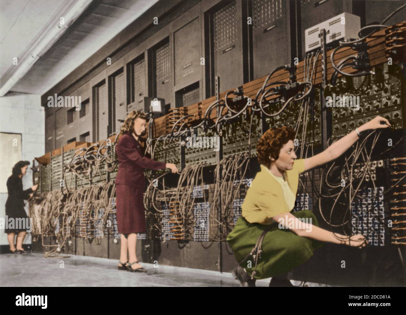
Placeholder image for First Generation Computers: ENIAC or TIFRAC.
Key Features
Vacuum Tubes
Used vacuum tubes as primary electronic components, making them large and heat-generating.
Large Size
Often occupied entire rooms due to the size of components.
Machine/Assembly Language
Programming was done in low-level machine code or early assembly languages.
Heat Generation
Generated significant heat, requiring extensive cooling systems.
High Power Consumption
Consumed a large amount of electricity to operate.
More Details
Electronics companies began mass-producing these computers. In the US, IBM entered the field with the IBM 701 (1952), its first scientific computer; only 19 units of the 701 were sold. Its success led to related models (IBM 650, 704). By the late 1950s IBM had leased about 1,000 first-generation computers – testimony to the rapid growth of computing.
Similarly, Remington Rand's UNIVAC I (1951) helped spur business and government interest. By contrast, European companies like Ferranti (UK) and Bull (France) produced fewer machines (hundreds), often focusing on specialized government or industrial uses.
In India during this era, computing was just beginning. As an emerging nation, India had limited industrial capability and scarce foreign currency. Importing even one computer required government approval, so early Indian scientists both imported and built machines.
In 1953, physicist Samarendra Kumar Mitra at the Indian Statistical Institute (ISI) in Kolkata constructed the country's first analogue computer (demonstrated to PM Nehru). The first digital machine in India was imported in 1955: a British-made 16-bit HEC-2M computer (Hollerith Electronic Computer, Model 2) installed at ISI Kolkata.
That same year, R. Narasimhan led a team at TIFR (Mumbai) to design a homegrown computer. By 1960 India's first indigenous computer, TIFRAC (vacuum-tube, 1956–1960), was completed. It used about 2,700 tubes and ferrite-core memory, and was formally dedicated in 1962.
However, the pace in India lagged far behind the West: whereas the U.S. built dozens of ENIAC-style machines, India had only a handful of tube computers by 1960 (TIFRAC being the largest).
Regional comparison: The USA dominated first-generation computing, with government and universities funding dozens of machines. Britain's efforts (Manchester, Cambridge, Ferranti) were fewer but influential. Continental Europe and USSR had a few projects (e.g. MESM in USSR, Telefunken in Germany). By contrast, India's first generation work started later and on a smaller scale.
Imported machines (British, American) mainly supported academia (ISI, TIFR, IITs) and government (bureaucratic data processing). A licensing regime and foreign-exchange shortage ("Licence-Permit Raj") meant India had to push for domestic development (e.g. TIFRAC) early on, even as it struggled to import technology. Overall, India built only a couple of dozen first-gen machines by the end of the 1950s, compared to hundreds globally.
References: Key sources include historical summaries of early computers, IBM product histories, and India-specific accounts. These provide the factual basis for dates, technical details, and comparisons.
3D Model Placeholder: Vacuum Tube or Early Computer Component
History and Milestones
1946
ENIAC (USA) completed – the first large, all-electronic general-purpose computer.
1949
EDSAC (UK) runs first programs; Manchester Mark I also operational.
1950–53
Several U.S. machines (UNIVAC I, IBM 701) and Soviet machines (BESM-1) become operational. Grace Hopper develops first programming languages/assemblers.
1953
At ISI (Kolkata), S.K. Mitra builds India's first analogue computer.
1955
HEC-2M arrives at ISI Kolkata as India's first digital computer.
1956
Design of TIFRAC begins in Mumbai.
1959–60
TIFRAC fabrication completes and enters service.
Late 1950s
Vacuum-tube computers in Europe and USSR; India remains primarily on imports and pilot projects.